 Richhiey Thomas
Inside SwiftF0: Architecture, Decoding, and Practical Capabilities
SwiftF0 is a compact neural fundamental-frequency estimator designed for monophonic audio. Its interesting idea is not simply that it is “small” or “fast.” The model reorganizes the pitch-estimation problem before applying a neural network: it converts waveform audio into a deliberately narrow spectral representation, learns local harmonic patterns with five convolutional layers, projects them onto a logarithmic pitch axis, and then decodes a continuous frequency from a local probability distribution. This article follows that path end to end—from samples to pitch_hz and confidence—and examines what those outputs can and cannot tell us.
The architectural facts below come from the SwiftF0 paper and the authors’ Python and ONNX implementation pinned in the references. Paper-reported benchmark results are labelled as such; they are not presented as measurements reproduced for this article.
The estimation target
Fundamental frequency, or F0, is the repetition rate of a periodic sound source. A harmonic signal with F0 at 220 Hz may contain energy at 220, 440, 660, 880 Hz, and higher integer multiples. The fundamental does not need to be the strongest spectral component. Resonances, recording equipment, and the sound source itself can make an upper harmonic larger than F0; the fundamental can even be weak or absent while the harmonic spacing still implies its period.
SwiftF0 is a monophonic estimator. It seeks one dominant F0 per analysis frame. That is different from polyphonic transcription, where several simultaneous fundamentals and note events may need to be inferred.
Pitch errors are naturally logarithmic:
The same absolute hertz error has a different musical meaning in different registers. A 5 Hz error near 100 Hz is much larger in cents than a 5 Hz error near 1 kHz. SwiftF0 therefore represents output pitch on a logarithmic axis and includes a log-frequency term in its training objective.
The complete signal path
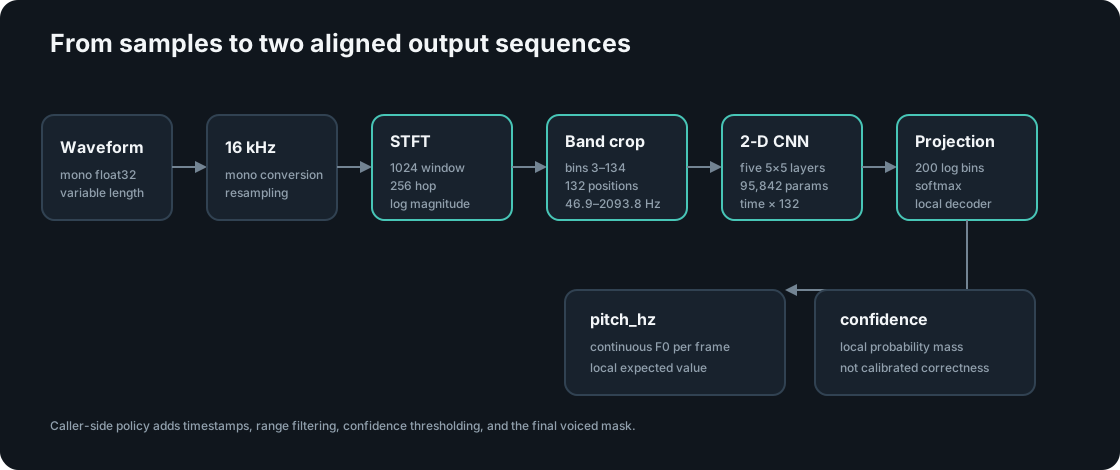
The reference package accepts mono or multichannel arrays at arbitrary sample rates. Package-level preprocessing averages multichannel input to mono and resamples it to 16 kHz when necessary. The ONNX model itself receives a floating-point waveform shaped as one batch by a variable number of samples.
The exported graph returns two aligned sequences:
pitch_hz:    one continuous F0 estimate per analysis position
confidence:  probability mass concentrated around the selected pitch peak
The Python wrapper derives two more arrays outside the model:
timestamps:  frame positions corrected for the model's STFT padding
voiced:      confidence and frequency-range threshold decision
This distinction matters. pitch_hz is an estimate for every output frame. Whether the application accepts that estimate as voiced is a policy decision applied afterward.
From waveform to a compact spectral representation
SwiftF0 operates at 16,000 samples per second. Its short-time Fourier transform uses:
| Quantity | Value | Consequence |
|---|---|---|
| Window | 1,024 samples | 64 ms of waveform context |
| Hop | 256 samples | One output position every 16 ms |
| Window function | Hann | Reduced spectral leakage relative to a rectangular window |
| Positive-frequency bins | 513 | 0 through 8 kHz before selection |
| Retained bins | 3–134 | 132 bins spanning the model’s pitch region |
| Linear bin spacing | 15.625 Hz | 16,000 / 1,024 |
For time index m and frequency index k, the paper defines the STFT as:
Here, N = 1,024 is the window length, H = 256 is the hop, and w is the Hann window. The complex STFT is reduced to magnitude, the selected frequency region is sliced out, and logarithmic compression is applied:
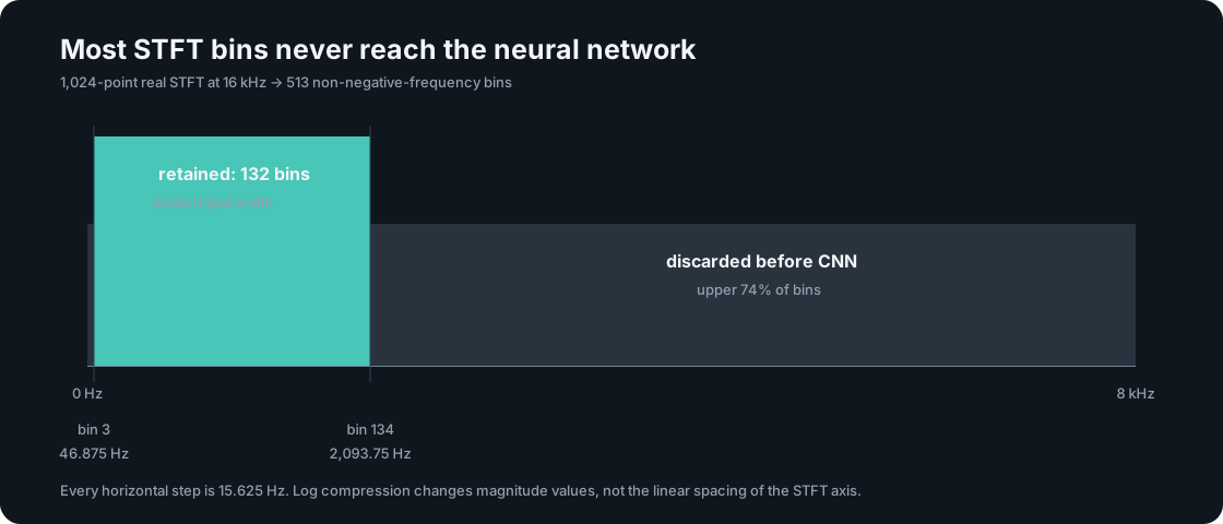
This crop is an architectural prior: the network is told where pitch-relevant spectral structure should be concentrated. It reduces the spatial width processed by every convolutional layer. It does not mean that overtones above 2.1 kHz never contain useful information, or that every sound inside the range is equally easy to estimate. The model deliberately trades broad spectral context for efficiency.
Five convolutional layers over time and frequency
The log-magnitude tensor has shape time × 132 frequency positions. SwiftF0 processes it with five same-padded 2-D convolutions:
channels:     1 → 8 → 16 → 32 → 64 → 1
kernel:       5 × 5 at every layer
stride:       1
activation:   batch normalization + ReLU after each convolution
padding:      “same,” preserving time and frequency dimensions
Stacking five 5×5 convolutions gives the final layer a 21×21 receptive field. Along the STFT frequency axis, 21 bins cover approximately 328 Hz. The paper’s interpretation is that this area is large enough to combine evidence from a fundamental and several nearby harmonics while keeping the architecture compact.
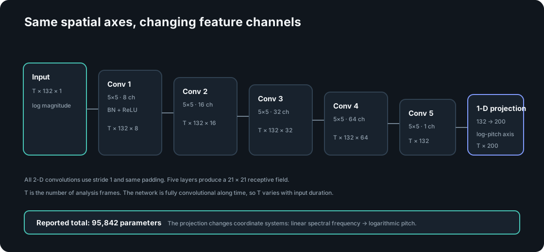
The paper reports 95,842 parameters for the complete network. Parameter count is not the same as execution time: runtime also depends on tensor sizes, operators, runtime implementation, CPU vectorization, threading, and input duration. Still, the small channel counts and cropped frequency axis explain why the model is structurally lightweight.
From linear spectral bins to logarithmic pitch bins
STFT bins are uniformly spaced in hertz, but musical pitch intervals are ratios. SwiftF0 projects the CNN output from 132 linearly spaced spectral positions to 200 logarithmically spaced pitch bins.
The center frequency of output bin b is:
With fmin = 46.875 Hz and fmax = 2,093.75 Hz, adjacent bin centers are approximately 33.1 cents apart. This is a classification grid, not the final resolution of the estimator. Continuous decoding combines neighboring bins.
Walk across SwiftF0’s 200 pitch bins
Equal steps in bin index produce equal pitch intervals, not equal hertz intervals. The hertz gap therefore grows toward the top of the range.
Training for a distribution and a continuous estimate
SwiftF0 is trained with two objectives:
- Categorical cross-entropy encourages probability at the correct pitch bin.
- L1 loss in log-frequency space penalizes the distance between the expected frequency and the reference F0.
The paper sets their weighting coefficient to one. The classification objective gives the network a well-structured output space; the continuous term discourages a correct-but-quantized solution that always collapses onto one bin center.
This is an important design choice. If the target falls between two bins, a useful distribution can place most probability on the nearest bin and some on its neighbor. The decoder can then recover a value between the centers. The output vector is therefore not merely an intermediate artifact—it is the representation from which both frequency and confidence are derived.
Local expected-value decoding
For each time frame, the network produces 200 logits. The decoder:
- Applies softmax to obtain a pitch distribution.
- Finds the maximum-probability bin b*.
- Keeps a local window from b* − 9 through b* + 9.
- Renormalizes probability inside that window.
- Computes a weighted frequency estimate from the local bin centers.
- Sums the original probability mass in the window to obtain confidence.
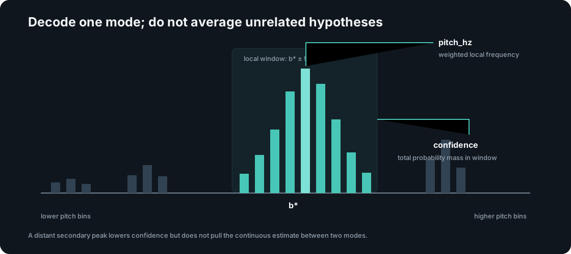
The local window prevents a distant secondary mode from pulling the estimate between two unrelated pitches. That is useful for octave ambiguity: averaging equal peaks one octave apart would produce a frequency that corresponds to neither hypothesis. Local decoding chooses one mode, then refines within it.
Confidence should be interpreted narrowly. It measures concentration around the selected mode under this model and training procedure. It is not guaranteed to equal the empirical probability that the estimate is correct, and thresholds may need validation for a specific domain.
What the released API outputs
The Python package returns a PitchResult with four aligned arrays:
from swift_f0 import SwiftF0

detector = SwiftF0(
    confidence_threshold=0.9,
    fmin=46.875,
    fmax=2093.75,
)
result = detector.detect_from_array(audio, sample_rate)

result.timestamps   # seconds
result.pitch_hz     # continuous model estimate
result.confidence   # local probability mass in [0, 1]
result.voiced       # wrapper threshold/range decision
The default voiced mask is:
confidence > 0.9
and pitch_hz >= fmin
and pitch_hz <= fmax
Changing fmin or fmax in the wrapper does not retrain or narrow the model’s physical output range; it changes which estimates are accepted as voiced. Likewise, lowering the confidence threshold trades fewer missed voiced frames for more false voiced detections. Threshold selection is part of the application, not an intrinsic model capability.
The package resamples non-16-kHz audio with librosa, averages channels for mono conversion, uses symmetric STFT padding of 384 samples, and timestamps frame i at:
The 127.5-sample offset accounts for the first window center after padding. It is about 7.97 ms. Correct timestamps matter when aligning SwiftF0 to annotations or to another detector; output arrays should not be compared by index when hop sizes or centering conventions differ.
Capability boundaries
The architecture supports several useful properties:
- Variable-duration waveform input through a fully convolutional time axis.
- One F0 estimate every 16 ms after framing.
- Continuous estimates between the 200 classification-bin centers.
- A confidence signal derived from distribution concentration.
- CPU inference through ONNX Runtime with one inter-op and one intra-op thread in the reference Python wrapper.
- A compact parameter count and an ONNX graph suitable for non-Python runtimes.
Those properties do not remove the limits of the task:
- Monophony: simultaneous fundamentals can create an ambiguous distribution.
- Frequency bounds: the exported model is constrained to approximately 46.875–2,093.75 Hz.
- Finite context: a 64 ms window limits temporal and low-frequency evidence.
- Spectral crop: useful upper harmonics above the retained band are discarded.
- Voicing calibration: confidence is not guaranteed to be calibrated across microphones, instruments, rooms, or noise conditions.
- Domain dependence: performance reflects the speech, music, synthetic data, and augmentations used for training.
- Streaming latency: a 16 ms hop does not imply 16 ms end-to-end latency. Capture buffering, resampling, required context, inference, scheduling, smoothing, and rendering all contribute.
Missing fundamentals, strong formants, note attacks, breath noise, vibrato, reverberation, and octave-related harmonic patterns remain difficult cases. A low confidence score can help suppress some failures, but suppression is not correction.
A compact browser deployment example
PitchSteps uses the SwiftF0 ONNX export as one selectable detector. At inspected revision ac0279b, microphone channels are averaged in an AudioWorklet, transferred in 2,048-sample batches to a Web Worker, linearly resampled to 16 kHz, and accumulated into 4,096-sample inference windows. The worker advances by 2,048 samples between calls.
onnxruntime-web/wasm loads the local model with one WASM thread and returns pitch_hz and confidence. PitchSteps then applies its own 80–1,000 Hz range, a 0.72 entry confidence threshold, a lower 0.60 exit threshold, level and clipping gates, continuity tracking, and a five-frame median filter before producing note and cents feedback.
This separation illustrates a general deployment principle:
model output          application interpretation
────────────          ──────────────────────────
pitch_hz       →      accepted range, note name, cents
confidence     →      voicing threshold and hysteresis
frame sequence →      continuity and display smoothing
The app can make the display more stable, but smoothing does not improve the raw model’s accuracy. It changes the behavior of the product built around the model.
Brief contrast with other learned F0 estimators
SwiftF0 belongs to the same broad family as learned, parametric pitch estimators, but its representation and efficiency priorities differ.
| Model | Input representation | Output geometry | Architectural emphasis |
|---|---|---|---|
| SwiftF0 | Cropped log-magnitude STFT | 200 logarithmic bins + local expected value | Compact frequency-domain CNN |
| CREPE | Raw 1,024-sample waveform | 360 bins at 20 cents + local weighted average | Larger waveform CNN; selectable capacities |
| PENN | Raw waveform-derived learned representation | Finer pitch classification and periodicity | CREPE-inspired efficiency and decoding refinements |
CREPE asks a deeper network to learn useful periodic structure directly from waveform samples. SwiftF0 makes the spectral transform and frequency crop explicit, reducing what the learned layers must process. Neither choice is inherently superior: waveform models retain fine temporal information, while spectral models inject a strong frequency-analysis prior.
The SwiftF0 paper reports 95,842 parameters and an average CPU time of 132.6 ms for five seconds of audio, versus approximately 22 million parameters and 5,508.3 ms for the TorchCREPE configuration in its benchmark. That reported 42.42× ratio is specific to the authors’ hardware, implementations, dependencies, and protocol. It is not a universal CREPE comparison and does not predict browser performance.
Conclusion
SwiftF0’s architecture is a sequence of deliberate reductions. A 16 kHz waveform becomes a 132-bin log spectrum; five small convolutions learn local time-frequency structure; a projection converts linear spectral positions into 200 logarithmic pitch hypotheses; and a local expected-value decoder turns one mode of that distribution into continuous F0 and confidence.
The most useful mental model is therefore not “a neural network that outputs pitch.” SwiftF0 is a compact probabilistic pitch representation with an application-facing decoder. Understanding the representation explains its efficiency, its between-bin precision, the meaning of confidence, and the places where downstream voicing and smoothing policy begin.
References and inspected revisions
- Nieradzik, L. “SwiftF0: Fast and Accurate Monophonic Pitch Detection.” arXiv:2508.18440, version 1, 25 August 2025.
- SwiftF0 source, commit
64700fc, retrieved 24 July 2026. - Kim, J. W., Salamon, J., Li, P., and Bello, J. P. “CREPE: A Convolutional Representation for Pitch Estimation.” arXiv:1802.06182.
- Original CREPE implementation, commit
c9b71ce. - Morrison, M. et al. “Cross-domain Neural Pitch and Periodicity Estimation.” arXiv:2301.12258.
- PitchSteps source, commit
ac0279b, retrieved 24 July 2026. docs/swiftf0-evidence-ledger.md, claim-level provenance for this article.